Results from a lab designed for preperation to work on our case study.

2. Write down the QG Geopotential tendency equation, and briefly discuss how each of the plots relate to the different terms in the equation.

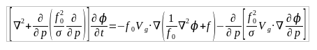
The first term of the equation is the geostrophic vorticity advection. The plot of the geostrophic vorticity advection at 500 mb uses this to find the areas that are experiencing the highest geostrophic vorticity advection. The second term is the temperature advection. Our plot of the differential temperature advection uses this part, but takes the differential of the temperature advection. 3. What was/were the dominating factors in the deepening of the 500-mb trough/strengthening of the downstream ridge? One was a deep area of the differential temperature advection, which was located over the southern part of lake Michigan when the low pressure was at its strongest. Another factor in the deepening was an area of geostrophic vorticity advection just west of the area that was seeing the worst weather at 18z. At its peak strength, the vorticity split into two areas. One was located over central Michigan, and the other was located over east central Illinois and western Indiana. 5. Write down the QG vorticity tendency equation (QGVTE), and briefly discuss how each of the plots relate to the different terms of the equation. What conditions would cause a lot of (b)?

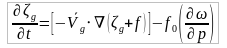
The 1000 mb geopotential absolute vorticity relates to the first term of the equation. This term is the advection of absolute geostrophic vorticity by the geostrophic wind. We use the geostrophic vorticity and the geostrophic wind to find it. The plot of differential omega is plotted using the last term of the equation, which is the vertical stretching term. The omega parameter is the top term of this term. We’d use this to find the omega, then take the differential of that to find the differential omega. The geostrophic vorticity advection at 1000 mb is directly related to the second term of the equation. That term is how we find the geostrophic vorticity advection, using the height given (1000 mb) and using the geostrophic wind for the plot as well. The biggest factor in the increased “spin-up” for the low was a high factor of geopotential absolute vorticity as the low tracked to the northeast. At 18z, the low was in an area that had a number of 30 s-1 for the geopotential absolute vorticity. As it tracked to the northeast, the vorticity in the area of the low deepened to 45 s-1.

This is an image of the 6 hou differences in geopotential heights between 18z Sunday (12 pm Sunday) and 0z Monday (6 pm Sunday). The red contoured lines show the areas of equal decrease or increase in the geopotential height field. (Made with gempak)

This is an image of the 500 mb geopotential heights at 18z (12 pm Sunday). The red contoured lines are areas of equal height values. (Made with gempak)

This image, much like the last one, is geopotential heights at 500 mb. FOr this image, the time is at 0z Monday (6 pm Sunday. The small dip seen in the heights is attributed to the cold front being in that area at that time. (made with gempak)

This is the differential temperature advection at 18z (12 pm) Sunday. The red lines show the advection of differential temperature. The biggest area is in southwest Missouri.(made with gempak)

This is a plot of the differential temperature advection at 0z (6pm Sunday) for the US. The red lines show the advection of differential temperature. The highest values are lagging back in the western plains. (made with gempak)

This is a plot of the geostrophic vorticity advection at 18z on Sunday. The red lines are lines of equal advection of geostrophic vorticity. Of note is the maximum in west central Illinois, along with the minimum right behind it. (made with gempak)

This is a plot of the geostrophic vorticity advection at 0z Monday The red lines show the advection of geostrophic voriticity. The maximum associated with the storm in question was located over East-central Illinois and western Indiana. (made with gempak)

This plot shows the geopotential absolute vorticity at 18z (12 pm Sunday) at 1000 mb, or at the surface. The red contured lines show the areas that are experiencing the highest values in geopotential absolute vorticity. (made with gempak)

This plot shows the geopotential absolute vorticity at 0z monday (6 pm Sunday) at 1000 mb, or at the surface. The red contoured lines show the areas that are experiencing the highest values in geopotential absolute vorticity. (made with gempak)

This plot shows the Differential omega at 18z on Sunday between 850 and 500 mb. These show the areas that will be experincing enhanced lifting due to the omega term. (made with gempak)

This plot shows the differential omega for 0z monday (6 pm sunday) between 850 and 500 mb. These show the areas that will experience enhanced lift due to the omega term. (made with gempak)