| Introductory Page | Conclusion of the case study | Case study prep lab |
|---|
This is the large scale pattern, along with the synoptic (regional) scale of the storm system.
3. Large Scale Pattern
The polar jet stream stretched across the central Mississippi river valley back to Texas, and back into the Pacific Northwest at 250 hPa at 0Z, as seen in Figure 5a. Meanwhile, the subtropical jet was stretching from the panhandle of Texas and Oklahoma, through Southern Illinois, and along the Ohio River valley. The subtropical jet exited the Conus around Outer Banks of North Carolina, and Virginia. The speed max, at 162kts, for the subtropical jet stream was located over southern Missouri. A second speed max in that segment of the jet stream over the state of Kentucky at 146kts as seen in Figure 5b. As the day went on, the polar jet formed more of the dip in the CONUS, with the main jet streak that provided our severe weather centered over west central Illinois.
The polar jet dipped down into the central Great Plains, and stretched back over the Rocky Mountains, and back into British Columbia at 12Z on the 17th as seen in Figure 6a. A small speed max of 122kts was seen over the southern portion of Kansas. The polar jet stretches from Canada, to the southeast over the American Rocky Mountains. The subtropical jet stretched from Oklahoma through southern Illinois and back into the Ohio River valley and Mid-Atlantic states, exiting the CONUS over the Delmarva Peninsula. It appears that the jet streams were phased together over the southern Great Plains and through the eastern portion of the CONUS, were there was a jet max of 136 knots over the Appalachian Mountains of West Virginia, as seen in Figure 6b.
The influence from the jet stream rapidly deepened the surface low pressure as it tracked to the northeast, into the southeastern portion of Iowa. As the jet streak moved to the northeast, by 12Z on the 17th, the left exit region of the jet streak was over west-central Illinois. This helped to increase the upper level divergence that the western part of Illinois was experiencing. The divergence helped to strengthen the low pressures as the moved to the northeast across the northwestern corner of Illinois. A jet max of 111kts was over the southwestern corner of Missouri. By 0Z on the 18th, the leading edge of the jet at 250 hPa had reached the southern shore of Lake Huron. A jet max of 124kts was seen trailing behind with the exit region of the jet streak over the eastern portion of the state of Illinois.
To the north of this, there was an upper level trough of low pressure in central Canada. The area in question was on the southeastern the influence of the trough. Further west, a small ridge was seen over southern Nevada. Both of the jet streams, fused together over the central Great Plains, followed this dip in the geopotential heights, which means the associated speed max with the jet stream also followed the same path. The height contours were tightest over the Rocky Mountains and over into the central great plains of Kansas and Oklahoma, where the jet max for the 250 hPa was located. As mentioned, the jet max for the subtropical jet stream was located over southern Missouri at 0Z, with the strongest part of the subtropical jet located over the northern part of West Virginia.
An upper level trough of low pressure formed over the upper peninsula of Michigan by 0Z on the 18th at 250 hPa, as seen in Figure 6c. The trough began to become slightly negatively tilted, causing the kinetic energy in the base of the trough to increase. At the same time, the subtropical jet that had been over the central Great Plains moved over the Outer Banks of North Carolina, and then out over the Atlantic. An upper level trough is seen over the southern part of Ontario. The jet stream at this level is not nearly as well defined as the earlier part of the day. There are still areas of faster winds, as evidenced by the area of 100kt plus winds at the base of the trough trailing behind the surface frontal boundaries. By 12Z on the 18th, the upper level trough of low pressure had pushed well into the northern part of Ontario. The jet stream at 250 hPa had become a bit less well defined. The low pressure, by this time was situated just south of Hudson Bay, with the trailing occluded front curving from the low back to just to the north of the state of Maine.
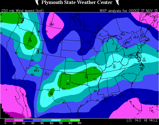
Figure 5a- This is the 250 hPa winds speeds in knots at 0Z on the 17th, contoured every 20 knots, with the green colors representing the higher winds, and the darker more purple colors representing the weakest winds. As noted, the jet stream was dipping from Canada and through the southern Great Plain states. Of note is the jet max located over the Idaho/Oregon eastern border. This would later come into play to help spark the convection. (Plymouth State)
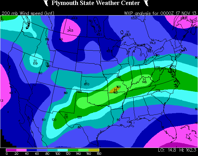
Figure 5b- This is the 200 hPa wind speeds in knots at 0Z on 17th, contoured every 20 knots, with the green colors representing the highest wind speeds, with the purple colors representing the slower winds. The subtropical jet is basically following the same path the polar jet was. Of note is the max over Wyoming. This would later help to get the convection to form. (Plymouth State)
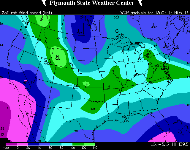
Figure 6a- This is the 250 hPa wind speeds in knots at 12Z, contoured every 20 knots, with green colors representing the highest winds, and the darker, more purple colors representing the weakest winds. As noted above, the jet is dipping down from Canada, into the Pacific Northwest, with two jet maxes behind the main jet streak. The left exit region of the jet was over the mid-Mississippi river valley. This would later help to spark the convection that would come. (Plymouth State)
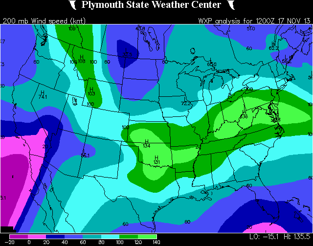
Figure 6b- This is the 200 hPa winds speeds in knots at 12Z, contoured every 20 knots, with the brightest colors representing the highest wind speeds, and the darker colors representing the slower wind speeds. The subtropical jet has moved over the center of the conus, and over into the western Atlantic. A speed max in the jet trails behind the main storm. This would help to enhance the damaging wind potential. (Plymouth State)
Synoptic/regional scale
The cyclone that caused this outbreak began to form on the lee side of the Rocky Mountains in the afternoon of November 16th. A warm front began to form at the same time. The warm front stretched from the low pressure, into west central Kansas, connecting into the cold front of the cyclone that impacted the Midwest on the 16th. A stationary front trailed behind the low pressure, which would later form into the cold front as it tracked into the Central Great Plains, as seen in Figure 7. The cold front that would cause the convection on the 17th began to form late in the afternoon of the 16th. The low, as mentioned earlier, was in the left exit region of a large jet streak. This caused the low pressure to rapidly strengthen as it moved to the east. The cold front associated with the cyclone that impacted the mid-Mississippi River Valley on the 16th took over the warm front that had formed earlier in the day. A mid-latitude cyclone with an associated occluded front was located over Minnesota at 0Z. Figure 8 shows this occuring. The cold front trailed back over central Iowa, through the northeast corner of Missouri, and into Kansas. Meanwhile, the cyclone in question was sitting in eastern Colorado, on the lee side of the Rocky Mountains. The cyclone began to move into the central Great Plains, with a warm front out in front of the storm as seen in Figure 8 as well. The cold front stretched behind, back into south central Colorado.
By 12Z, the cyclone had pushed into the east, into the northwestern corner of Missouri. The warm front stretched from the low pressure, through Iowa, and into northern Illinois. The cold front trailed behind from the low pressure, back into Kansas, Oklahoma, and the northern panhandle of Texas. By 15Z, the frontal system that moved through the Midwest on the 16th moved further to the northeast. The cold front stretched from central Missouri, back into Oklahoma. The main area of surface low pressure pushed into northeast Missouri. A second low pressure area formed in eastern Iowa at the western end of the warm front. The warm front at that time stretched through southern Wisconsin and over into northern Indiana. As the day went on, the mid-latitude cyclone rapidly moved to the north and the east, strengthening to 982 hPa by 6 pm on the 17th. The cold front by that time was paralleling the Indiana-Ohio boarder, with a low-pressure area was sitting over the west-central Michigan at the northern end of an occluded front. Over the eastern end of the Upper Peninsula of Michigan, a second low pressure sat at the western end of the warm front, which stretched from the low pressure, eastward into New York. The cyclone accelerated to the northeast, the warm front stretching from the north shore of Lake Ontario, back over northern New York, and back into the New England states. The cold front stretched from the occlusion point back through Pennsylvania, and back into Texas. An occluded front stretched from the low press back to the point of occlusion. The low pressure's central pressure fell to 971 hPa by 6Z on the 18th. By that time, the fronts were stretching from Canada, back through the northeast, and back through the south. The main low pressure became cut off from the warm air. This caused the cyclone to dissipate early in the day on the 19th. Figure 9 shows the dissipation of the occluded front, with the low well to the north of the intersection of the warm and cold fronts.
An upper level front is an area of temperature gradient and high static stability in the mid to upper part of the troposphere. It doesn't necessary have to extend down to the ground. At 12Z on the 17th, there was the beginnings of an upper level front over Colorado and New Mexico as seen in figure 10a. This was the upper level frontal system that was beginning to develop in the vicinity of the surface frontal boundaries. As the upper level front moved to the east, it became more noticeable by 12Z on the 17th. By that time, it was nearly co-located with the surface low pressure, as seen in figure 10b. The front gets even more noticeable by 0Z over the states of Michigan and Indiana. This was associated with the storm becoming occluded from its warm air supply. The upper level front continues to move eastward, now centered over Lake Huron at 12Z on the 18th. The occluded front, by this time, has become elongated with the triple point occurring just to the north of the border between Quebec and Maine, with the occluded front stretching from that intersection point, back northward to the south shore of Hudson Bay, as seen in figure 10c. The upper level front is still visible at 18Z on the 18th over the eastern shore of Lake Huron. The upper level front was absorbed into the tropopause, signifying the end of the cyclone, as the cyclone dissipated early in the day on the 19th.
There was a shortwave trough over the northern part of Colorado at both the 700 and 500 hPa pressure levels. The shortwave has rising motion on the exit area, and this was co-located with the surface low pressure, feeding it more rising motion to strengthen the cyclone, as noted in Figure 11a and Figure 11b. This added to the upward motion that was needed for the development of the severe convection. The shortwave rapidly moved into the Mid-Mississippi River valley by 0Z on the 18th as seen in Figure 11c. The upward motion from the shortwave helped to increase the upward motion that cyclone was experiencing, leading to rapid development of the convection. The strongest upward motion from the shortwave was pushed east southeastward, keeping the convection that formed over the Tennessee Valley strong as the environment lost the daytime heating.
The morning sounding from Lincoln, IL (KILX) showed significant low level speed and directional shear, as seen in Figure 12. Looking further up in the troposphere, the shear was primarily unidirectional in nature. This caused the convection to, initially, be of the supercell thunderstorm type. However, the storms became more linear in nature as the day went on. The sounding had the classic QLCS-type look with directional and speed shear in the lowest 100 hPa, with unidirectional speed shear further up. The shear in the lowest 100 hPa was veering with height, with winds out of the south at the surface, and winds at 900 hPa out of the southwest. Looking at the CAPE values, there was not a huge amount of CAPE that day. The value at KILX of CAPE at 12z that morning was only a little more than 900 J/kg. “HSLC events can occur at all hours of the day; however, an evening peak was noted in the diurnal cycle of HSLC significant severe events, with a mid- to late-morning minimum.” (Sherburn, Parker, 2014) This means that this type of environment is more common in the afternoon and evening of the day, rather than the morning time. The hodograph that was also produced showed a veering with height from the surface to 925 hPa, then a continued veering with height from there on up, as seen in Figure 13. “The mean soundings show progressively lower temperatures with increasing tornado intensity and a drier mid-troposphere for the F3 sounding.” (Colquhoun, Riley, 1996) This means that when there is a probability for tornadic formation, if there is a significant area of dry air in the upper portions of the atmosphere. We can assume that there was a significant area of dry air due to the fact that the threat for damaging winds was very high that day.
The major moisture source for this storm was the Gulf of Mexico. Out in front of the main system and cold front, a warm front lifted through the state, swinging the winds out of the south at the surface. By 15Z, dew points throughout most of the state was near 60 degrees. This can be seen in figure 14. Along the front and behind the frontal zone, the dew points rapidly fell as cold and dry air from Canada moved in. Immediately behind the front, there was a steep dew point gradient, as there normally is with a late season severe weather event. By 18Z, the 60 degree isodrosotherm was paralleling the US 51 corridor as the cold front swept through the state.
Looking at the visible satellite imagery, the overnight overcast and convection had moved out from the area by 14Z. At just before 15Z, towering cumulus and a small area of convection had begun to form out in Missouri along and ahead of the cold front, as seen in Figure 15. At 1715Z, the storms with several overshooting tops, were located basically along and west of interstate 55 in central Illinois. Out in front of the storms at that time, there was some clearing occurring downstream of the storms. This would help with downstream strengthening of the QLCS as it moved to the east, as noted in Figure 15. Behind the main line, a secondary line right ahead of the cold front moved into Illinois from Missouri and Iowa. As the day went on, the cold front swept through, sweeping the storms out along with it. This is seen in Figure 15.
While looking at the Infrared satellite imagery, we can see the convection that grew the tallest by looking at the coloration of the imagery as well as the advection of moisture. At 1515z, the convection in west-central Illinois began to grow into the vertical and the tops of the clouds turned cooler, as seen in figure 16. As the day continued, the tops of the convection reached into the -50°F area. This meant that the convection that was forming was growing huge in the vertical direction. With the storms being tall in the vertical direction, they could tap into the jet stream and the associated jet max associated with it. This would be a factor in the destructive straight line wind gusts that would affect the Chicagoland region and the downstream states.
Looking at the infrared water vapor imagery, there was a lot of clouds out in front of the storm. At 12Z, a band of convection is seen from Arkansas back over Indiana and Ohio, as seen in Figure 17. This caused the moisture that the storm had to use to be lessened. With less moisture for the storms to work with, the shear would dominate the day for the storm. At 15Z, the convection from early on the 17th, was seen to be along and just north of the Ohio River. This is evident by the dark blue areas where there is moisture being detected by the satellite. This is seen in Figure 17 as well, in frame 2. At 18Z, there is areas of blue in the water vapor imagery over the state of Illinois. This is when the storms were really taking off in intensity, tapping into the limited instability that they did have. This can be seen in Figure 17, frame 3.
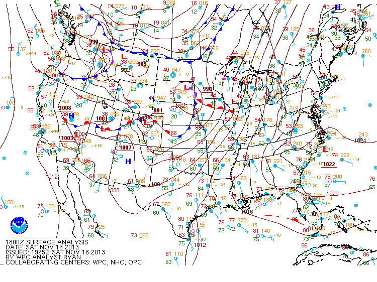
Figure 7- This is an image of the surface analysis at 18Z on November 16th. The mid-latitude cyclone that impacted the weather on the 16th was centered over South Dakota. At the same time, a low pressure began to develop on the Lee-side of the Rockies in north Central Colorado. This would later cause the convection that the Midwest would experience on the next day. (WPC)
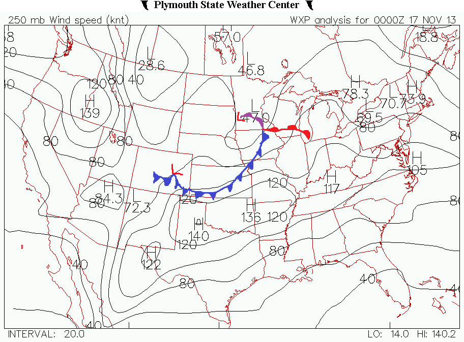
Figure 8- This is a gif depicting the positions of the jet stream and associated jet maxes and fronts, contoured every 20 knots for the time period between 0Z on the 17th The fronts are annotated on each image for the same time. Of note is the rapid speed at which the storm passes through. The rapid movement is due to the extremely high winds at upper levels propelling the storm along. (Plymouth State)
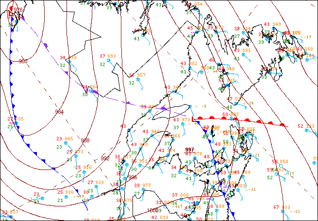
Figure 9- This is an image showing the surface analysis over eastern Quebec and the maritime eastern portion of Canada at 9Z on the 19th. As noted, the leading low pressure for the storm became completely cut off from its supply of warm air. This dissipated the occluded front. A second low would take over at the intersection of the old low pressure and the warm front. (Weather Prediction Center)
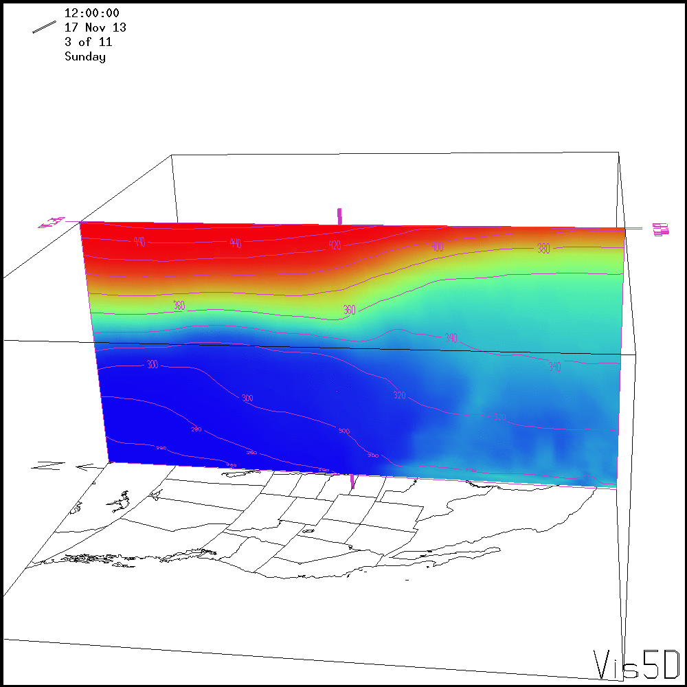
Figure 10a- This is a vertical slice of theta (the pink contours) and theta e (the colored vertical slice) at 12Z on the 17th. The brighter that the colors are, the higher that the value for theta e will be. Of note is the bulge beginning to form above eastern Kansas. This is the developing upper front that would add to the static stability behind the cyclone. (Vis5D)
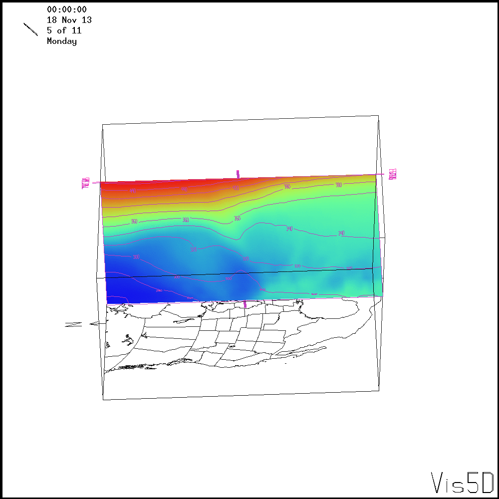
Figure 10b- This is a vertical slice of theta (pink contours) and theta e (colored vertical slice) at 0Z on the 18th. The upper front has gotten much more noticeable as the cyclone has moved to the east. With the strengthening of the upper front, this also means that there is a strong jet stream in the vicinity of the upper front. (Vis5D)
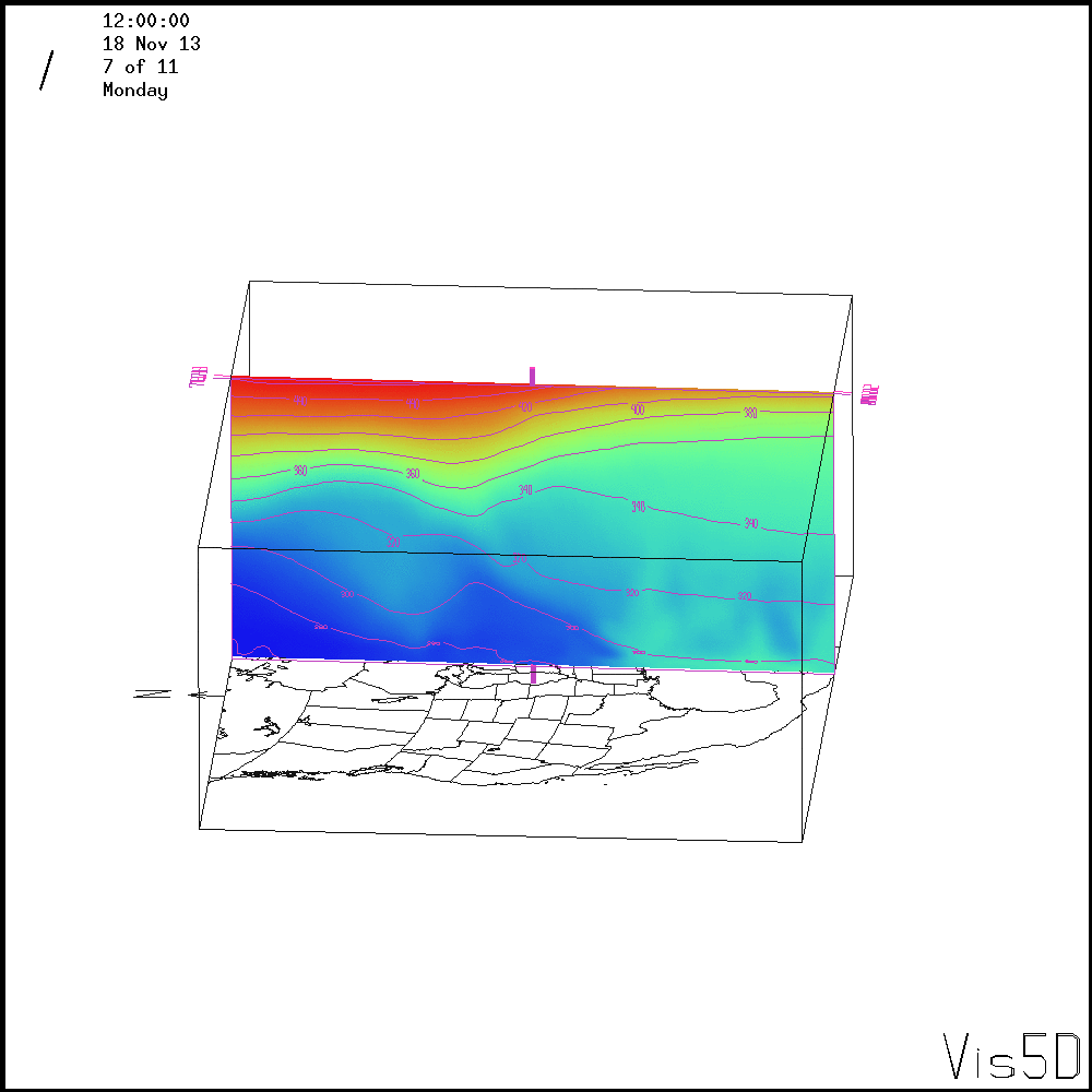
Figure 10c- This is a vertical slice of theta (pink contours) and theta e (colored vertical slice) at 12Z on the 18th. As noted, the upper level front began to weaken as it moved further away from the main jet stream. This also had a hand in the dissipation of the surface low and occluded front on the 19th. (Vis5D)
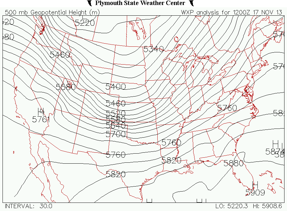
Figure 11a- This is the 500 hPa geopotential heights in meters, with a contour interval of 30. As noted, there is a shortwave over the foothills of the Colorado Rocky Mountains. The upward motion that is associated with the short wave is to the east of the shortwave. This would help to add upward motion downstream of the shortwave, which was the area thatwould see the convection later. (Plymouth State)
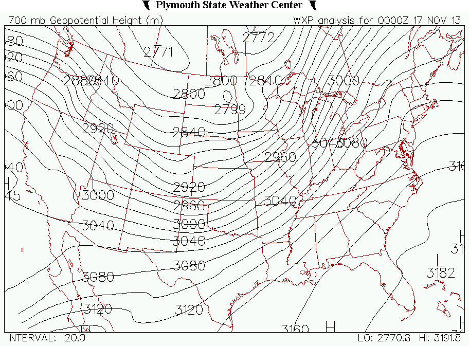
Figure 11b- This is the 700 hPa geopotential heights, in meters, with a contour interval of 20 meters at 0Z on the 17th. As noted, there is a shortwave over the northern part of Colorado and Wyoming. The upward motion, at the time, was located in the general area where the surface low had developed. This would later move eastward and have a hand in adding its upward motion to the storm. (Plymouth state)
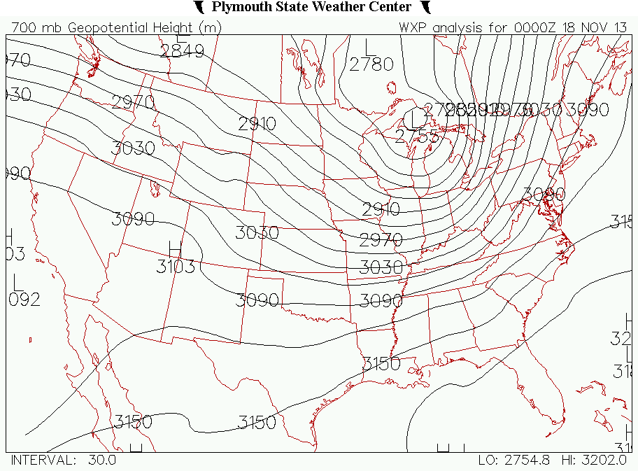
Figure 11c- This is the 700 hPa geopotential heights, in meters, with a contour interval of 30 meters at 0Z on the 18th. As noted, the short wave had moved its way to the area that the surface low pressure was at. This means that the shortwave had a hand in the deepening of the surface low as it moved to the northeast from Northern downstate Michigan. (Plymouth state)
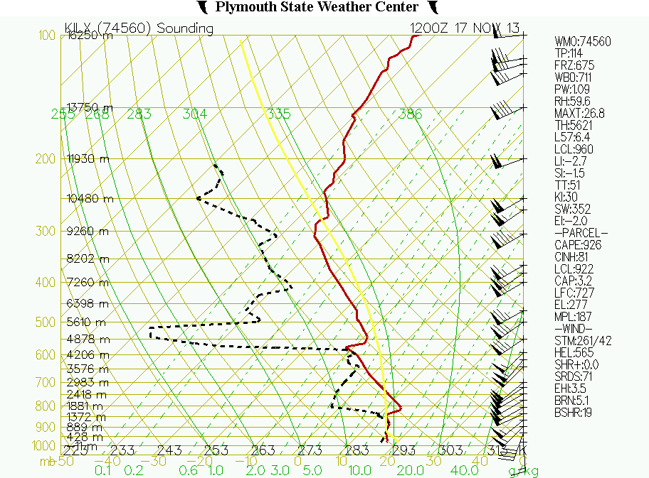
Figure 12- This is the Skew T sounding for KILX (Lincoln, IL) at 12Z on the 17th. As mentioned previously, there is significant lower level directional and speed shear. This is huge, mostly because there is a need for low lever shear with unidirectional shear above for the development of a QLCS. Of note is a wedge of dry air at 850 hPa. This would later help produce the significant damaging winds that would occur later. (Plymouth State)
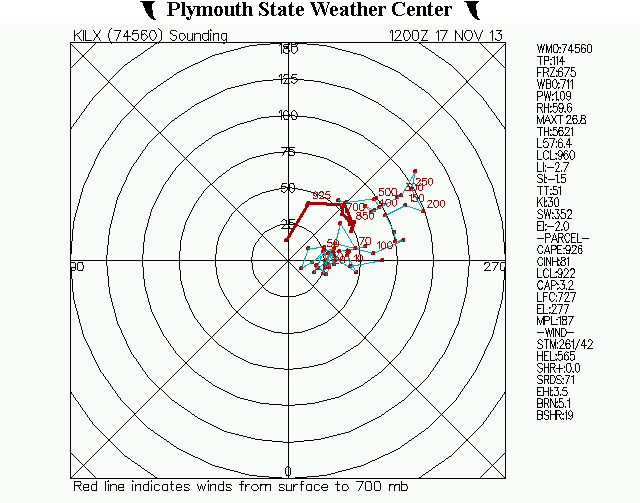
Figure 13- This is the hodograph for KILX at 12Z on the 17th. As noted, the winds were veering with height in the lowest 100 hPa of the atmosphere. This gave the storms significant low level shear, which is needed for the development of a QLCS type squall line. The winds further up are primarily unidirectional, consistent with the damaging wind threat. (Plymouth state)
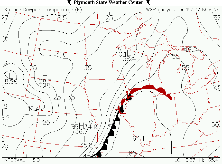
Figure 14-This is the surface dew points in Fahrenheit with the fronts annotated, from 15Z on the 17th. Each contour is an isodrosotherm, a line of constant dew point value, and has a contour interval of 5. As noted, the warm front associated with this storm system lifted through the state, which turned the winds to the south. This, in turn, would help to create more shear. Further north, the 55 degree isodrosotherm stretched all the way into northern Michigan. The overrunning moisture would cause elevated convection in the area. (Plymouth State)
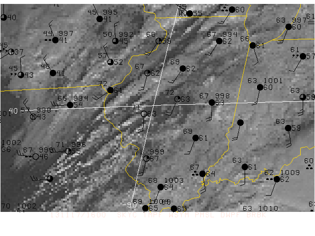
Figure 15- This gif is a series of images depicting the visible cloud cover and observations from 1545Z (first image), 1715Z (second image), and 1915Z (third image). Of note is the short clearing of the clouds that appeared at 1545Z. This would cause the temperatures to climb, and cause the instability that we did have to climb. It would lead to the strengthening of the convection. (GEMPAK)
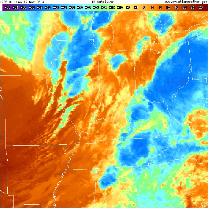
Figure 16- This is an infrared image of the cloud structure at 1725Z on the 17th. The red colors are where the temperatures are the warmest or where there are not any deep or noticeable clouds. The darker blue colors are the cloud tops that are colder. Of note is the tops reaching down into the area around -45 degrees. The cooler that the tops are, the taller that the convection is. This means that the convection can tap into the upper level winds, and the divergence that was seen over the area can also enhance the convection as well. (aviationweather.gov via UCAR's archive)
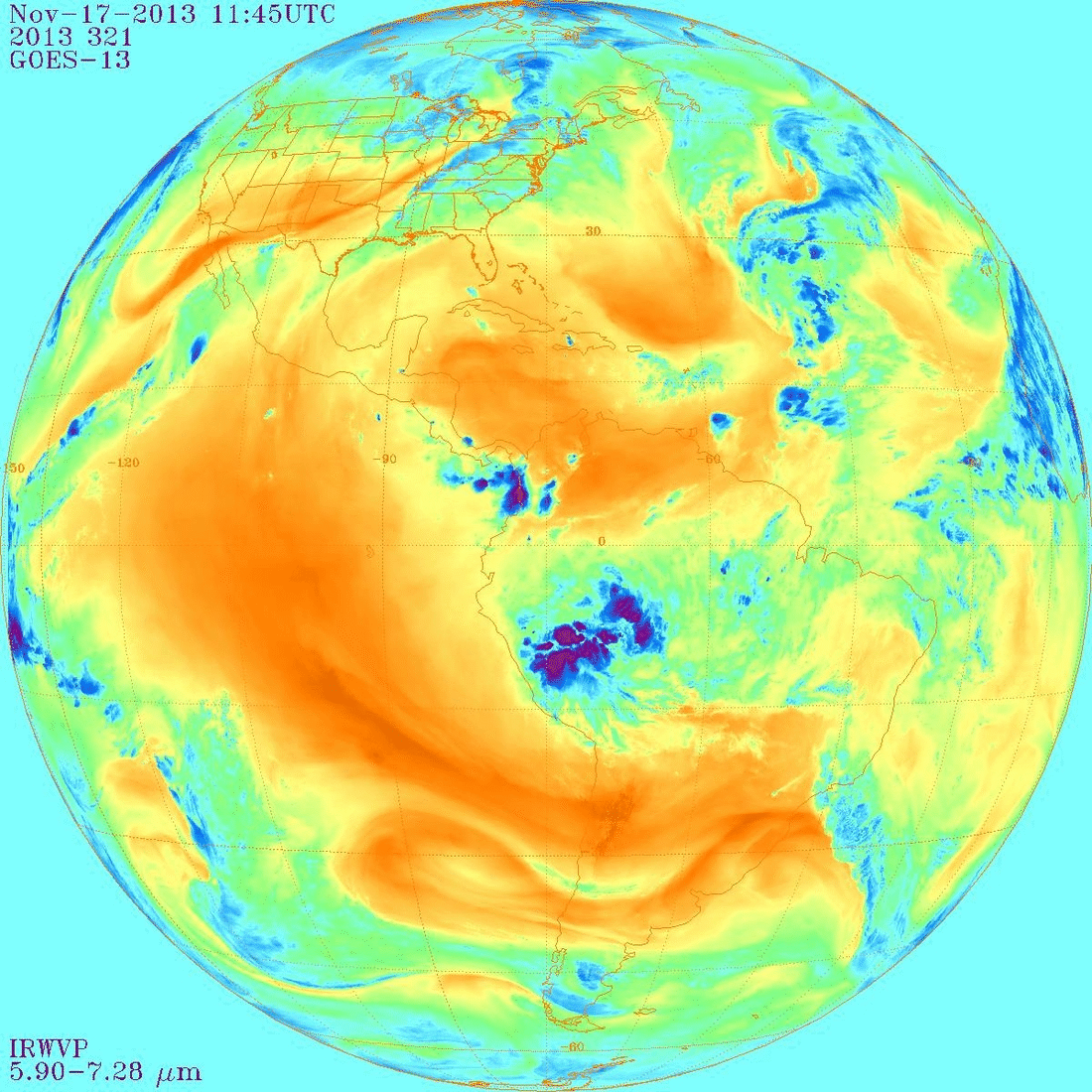
Figure 17- This is a gif of infrared water vapor imagery. The brighter colors mean that the water vapor in that area is warmer. The darker blues mean that the water vapor in that area is colder. As mentioned, the dark areas in each frame are clouds with colder tops. This means that the storms were getting fairly large in the vertical sense. This would help in the ability for the storms to bring the damaging wind gusts down from the upper levels to the ground. (NCDC)
5. Jet streaks, as we have learned before, have divergence in the right entrance and the left exit regions. There are areas of convergence at the left entrance and right exit regions. The convergence limits the strengthening of the surface low pressure as it sits below it. At 0Z on the 17th, the right exit region of the main jet streak that affected the mid-latitude cyclone was sitting over the Pacific Northwest, with the left exit region of the jet streak sitting over the Idaho-Montana boarder. At the south end of the dip in the jet stream, there was another jet streak. The right exit region of this jet streak was located over the state of Missouri, with the left entrance region of this jet streak in the general vicinity of the left entrance region of the departing jet streak. This limited the strengthening of the low pressure temporarily, as seen in Figure 18a. However, the first jet streak moved over the Delmarva Peninsula. The second jet streak then moved into the great plains and the Mid-Mississippi River valley. The low pressure, as shown earlier, was in the general vicinity of the right exit region at 12Z. The jet streak's right exit region sits generally just to the northwest of the surface low. There is clear divergence in the wind contours at that time as seen in Figure 18b. The surface low pressure moves into a more favorable position as it moves to the northeast at 0Z on the 18th. The two surface low pressures moved into the left exit region, where there is clear divergence in the wind contours. This is over the northern and central part of Michigan. This can be seen in figure 18c. The jet streak would then flatten out, with another jet streak trailing behind the surface cold front.
The short wave, as mentioned in the previous section, are rapidly moving small dips in the geopotential height fields, generally visible at 500 hPa. It has upward motion on the rear flanks. So, as the short wave passes, the upward motion will be on the backside of the shortwave. The short wave for this storm was located over the state of Wyoming at 12Z on the 17th. As the day went along, the short wave moved into the Mid-Mississippi River valley by 0Z on the 18th. The short wave was trailing just behind the cyclone, not helping to add to the cyclone. This can be seen in Figures 11a-c.
Surface temperature gradient is the quantity that describes the direction and rate of a temperature change, usually with the units of degrees per unit length. This is the strongest when in the vicinity of a frontal system. At 0Z on the 17th, there is a tight temperature gradient in Colorado, back into northern New Mexico. This area of the surface temperature gradient is due to the developing surface fronts. An area of CAA is seen behind the high surface temperature gradient. To the southeast, there is evidence of a warm front forming as there is an area of WAA occurring out in front of the developing fronts. The temperature gradient is moving to the south and east along and just behind the surface fronts. With the fronts moving to the east, the surface temperature gradient moved eastward as well. This caused at least some instability to build, even with the more limited moisture that was in place in the morning. This can be seen in Figure 19. The gradient got tighter as the mid-latitude cyclone strengthened. The southerly winds out in front of the storm strengthened the temperature gradient further. This was because the southerly winds sent warmer air from the deep south into the mid-Mississippi River Valley. This, in turn made for a strengthening of the gradient as the cyclone moved to the east. At 18Z, the tightest gradient of temperature is located in mid-Mississippi River valley. It's associated with the eastward propagation of the cyclone. The cold front, which at that time was located over the Illinois River Valley, is causing some WAA, as evidenced by the 70-degree contour reaching into southern Illinois. This can be seen in Figure 19b. The temperature gradient became a bit weaker as it got later in the night, due to the loss of the daytime heating. The tightest gradient of temperature is over Illinois where the wind out of the northwest are causing CAA to occur over the region, as seen in Figure 19c.
The thermal wind is a wind shear that flows parallel to the thicknesses, and is a function of how strong the temperature gradient is. The tighter that the thickness gradient is, the stronger that the thermal wind will be. At 0Z on the 17th, the strongest area of thermal wind is over central Kansas, and back into Colorado, where the cyclone is at that time. This means that this area, as mentioned above, is experiencing the strongest temperature gradient. The strongest area of thermal wind moved to the east as the front moved through the central Great Plains. The components of the wind (U and V) resulted in the thermal wind all along the 1000-500 hPa thicknesses. At 12Z on the 17th, the tightest gradient of the 1000-500 hPa thicknesses occurred over the mid and upper Mississippi river valleys. The thermal wind is out of the southwest generally, meaning that the u and v components are out of the north and west respectively. At 0Z on the 18th, the most significant thermal wind was seen over Indiana and southern Illinois. This means the temperature gradient was quite significant at that time. The thermal wind over this area was generally out of the south and southwest. This caused the air out in front of the storm to rise, according to the relation between the QG-omega equation and the rising motion associated with the storm. This is seen in Figure 20.
When looking at the upper level divergence, we're looking for the areas where the wind pulls apart from each other. Meaning, we're looking for areas where the wind diverges into different directions. In the area that has the divergence, this is the area where there will be convergence at the surface. When there is surface convergence, this is the area to look at for upward motion, as upward motion is one of the things needed for the development of convection. At 0Z on the 17th, there is some divergence over the Four Corners region, with the streamlines spreading apart there, as seen in Figure 21a. The wind for the most part otherwise over the Conus is in a zonal pattern. At 12Z the divergence of the wind streamlines became more obvious over the mid-Mississippi river valley. The dip in the jets is seen above, with convergence of the streamlines behind the divergence on the western side of the dip of the jets. At 0Z on the 18th, this divergence in the upper levels has moved to the east and is centered over Michigan. This was the area where the surface low was located. The upward motion was also located over this general area, as seen in Figure 21b. By 12Z on the 18th, the divergence had split into two areas. One area of divergence was seen over eastern Quebec, associated with the warm and occluded fronts, along with the upper level low that was sitting over eastern Ontario. The second area of divergence was associated with the jet streak that was mentioned earlier in the paper, which is occurring over the mid-Atlantic states. This was the area that was experiencing the most upward motion, with the front in the same area.
Vorticity is the amount of spin in a parcel of air. This is the second part of the QG-omega, with the positive vorticity advection being proportional to the rising motion. On the east side of a vorticity maximum, there will be upward motion that will help in the deepening of low-pressure and formation of the convection. West of the max, there is downward motion. In the Figure 22a, the vorticity advection was occurring over Colorado. At the same time, there was an area of 500 hPa absolute vorticity sitting over northern Kansas. In Figure 22b, there is a large area of positive vorticity advection occurring over the western portion of the state of Illinois at 18Z on the 17th. At that time, the surface low pressure was at the northern end of the maximum. As the afternoon continued onward, the vort max at 500 hPa moved eastward, and split into two distinct regions. The northern region of vorticity advection was associated with the low pressure systems, while the southern region was associated with the frontal boundary, as seen in figure 22c. At 1000 hPa, there is a maximum of absolute vorticity in the vicinity of the low. The low was on the eastern flanks of the vort max, and thus under the influence of the upward motion from the maximum according to the QG-vorticity equation, as seen in figure 22d. The vort max at 1000 hPa moved its way into the northern part of the state of Illinois, out in front of the storm. A second maximum in absolute vorticity was located to the north of where the frontal system was located. This area to the north helped somewhat to deepen the low more, but it was mostly the forcing from the jet streak that I mentioned earlier that helped to deepen the low at 12Z that day. Continuing into the 18th now, a vort max was parked just to the south of the double barrel low pressure systems to the north. A second max was just behind the first maximum, helping to deepen the low pressures as the system moved to the north and east, as seen in Figure 22e. By 12Z on the 18th, the vorticity max had moved out in front of the surface low. This means that the low was seeing the downward motion on the backside of the vorticity maximum. This was one of the keys in the dissipation of the surface low, along with the elongation of the occluded frontal boundary.
With isentropic lifting, the lifting can be found by looking in the areas that warm air advection is occurring. For my case study, I used the 300 Kelvin isosurface. At 18Z, there is an area of isentropic lifting to the north of the warm front that was snaking its way through the northern part of Illinois. This was the area that was just north of the warm front. (Figure 23a) By 0Z, the isentropic lifting that was occurring with the cold front intensified as the surface low intensified. The strongest area of isentropic lifting is occurring just to the north of the warm front, where overrunning of moisture and warm air advection is occurring at the same time. This had some hand in the deepening of the storm, as the WAA fed the low with warm air needed to deepen the surface low. (Figure 23b)
The main source of the ageostrophic motions was from the large jet streak that was sitting over the western portion of Illinois as the low pressure at the surface was deepening. This was the area that was experiencing divergence at the left exit region of the jet streak. As we previously learned, divergence of the wind is a function of the ageostrophic wind. This is due to the geostrophic wind having zero divergence. The divergence of the wind moved to the northeast as the surface frontal system did so, helping to deepen the low even further. The ageostrophic motion from the jet streak went further south, heading out over Atlantic as the day continued. However, a second jet streak moved its way over the central portion of the state of Illinois. This added some ageostrophic motion to the storm due to the divergence of the winds at 200 hPa. This jet streak had a direct hand in the deepening of the surface lows at the moved to the northeast into eastern Canada. (Figure 24) Omega, a measure of rising or falling of the air, is a major contributor to the QG-Omega equation. IN the areas at is experiencing advection of omega, these areas would be experiencing enhanced upward motion. Between 850 and 1000 hPa at 12Z, the highest amount of omega was found to be in the northern parts of Illinois. However, there was a lobe of omega building up in the mid-Mississippi river valley. (Figure 25a) Between the 850 and 500 hPa levels, there are two distinct areas of omega at 0Z on the 18th. One is in downstate Michigan with another stretching through the southern portion of Illinois, back into southern Oklahoma. (Figure 25b)
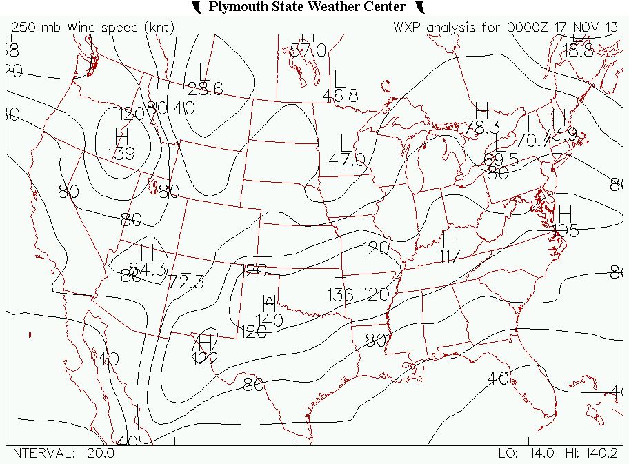
Figure 18a: This is the 250 hPa wind speed in knots, with an interval of 20 knots, at 0Z on the 17th. As noted, the left entrance region of the jet streak that was at the base of the trough was near the area that the surface low pressure had formed. Of note is the high jet max over the pacific northwest. This would cause the surface low to deepen later in the day. (Plymouth State)
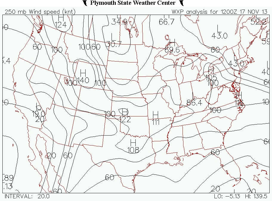
Figure 18b: This is the 250 hPa wind speed in knots with an interval of 20 knots, at 12Z on the 17th. As noted earlier, jet streak that was as the base of the trough moved out over the western Atlantic. The jet max that was located over the pacific northwest moved southeast into the Midwest of the US. Of note is the divergence just to the north of the jet stream and jet streak. The low pressure was sitting under this general area, strengthening it. (Plymouth State)
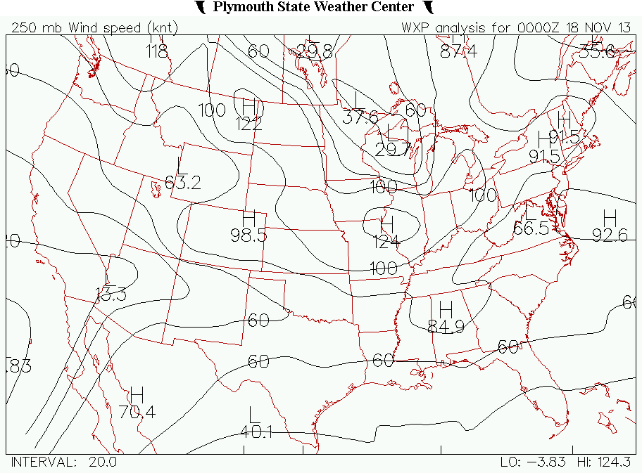
Figure 18c: This is the 250 hPa wind speed in knots at 0Z on the 18th. The contour interval is 20 knots. The left exit region of the jet stream was, at that time, located over the northern portion of Michigan. The surface low as under a clear area of divergence there. This caused the low to deepen as it pushed northeastward. (Plymouth State)
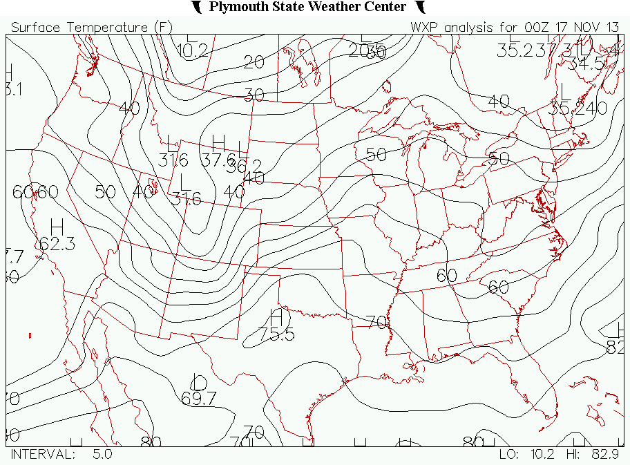
Figure 19a: This is a map of surface temperature in Fahrenheit at 0Z on the 17th, with a contour interval of 5 degrees. At that time of the day, the gradient was the tightest from Central Kansas and back through the northwestern corner of the panhandle of Texas. Of note is where the 60 degree isotherm is. This was the approximate position of the warm front that evening, with the cold front trailing back into the great plains. (Plymouth State)
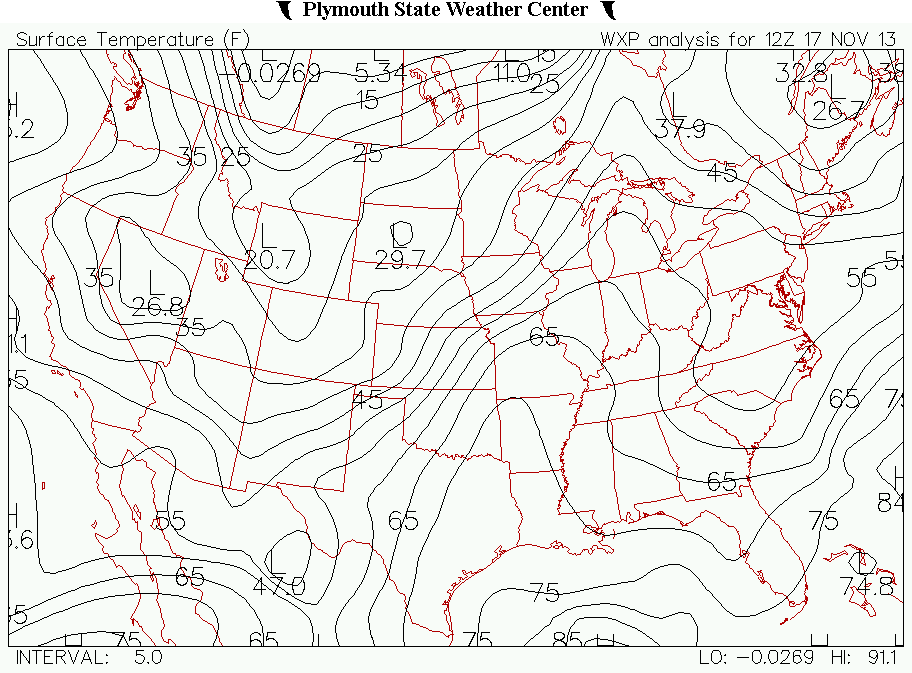
Figure 19b: This is a map of surface temperature in Fahrenheit at 12Z on the 17th, with contour interval of 5 degrees. Of note is the tightness of the temperature gradient in Missouri and Kansas. This is where the cold front was at that time, with the warm front stretching to the northeast along the 60 degree isotherm. (Plymouth State)
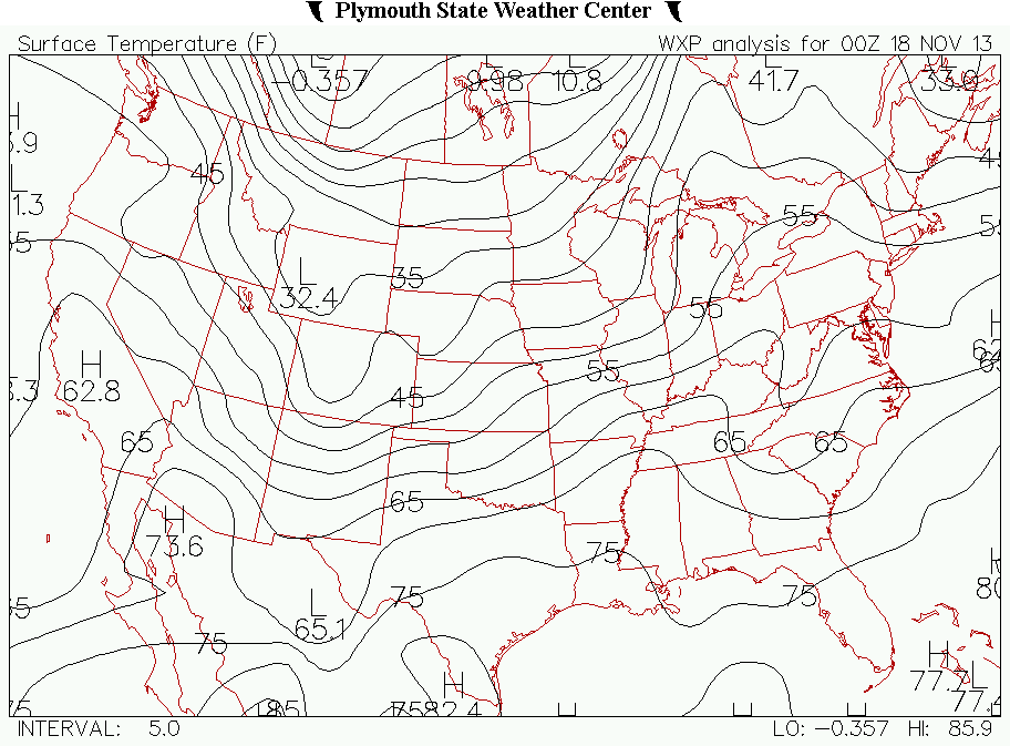
Figure 19c: This is a map of surface temperature in Fahrenheit at 0Z on the 18th, with a contour interval of 5 degrees. The earlier temperature gradient has laxed a bit as the area lost the heating from the day. Still, there is a temperature gradient stretching north-south through the state of Illinois. (Plymouth state)
.gif)
Figure 20: This is a gif animation of the 1000-500 hPa thicknesses from 0Z on the 17th through 0Z on the 18th. The interval of the contours is 20 meters. Of note is the strengthening of the thickness gradient at 0Z on the 18th. This was associated with the strengthening of the surface low pressure as it moved to the northeast (Plymouth state)
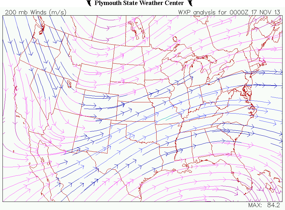
Figure 21a: This is a map showing streamlines, which shows the direction from which the wind is coming from and going to. The coloration basically shows where the wind is going faster or slower. At 0Z on the 17th, there is some divergence occurring over the northwestern corner of Arizona. Of note is the area of divergence that is occurring over the western portion of the state of Kansas. This was preventing the low from deepening much that evening. (Plymouth state)
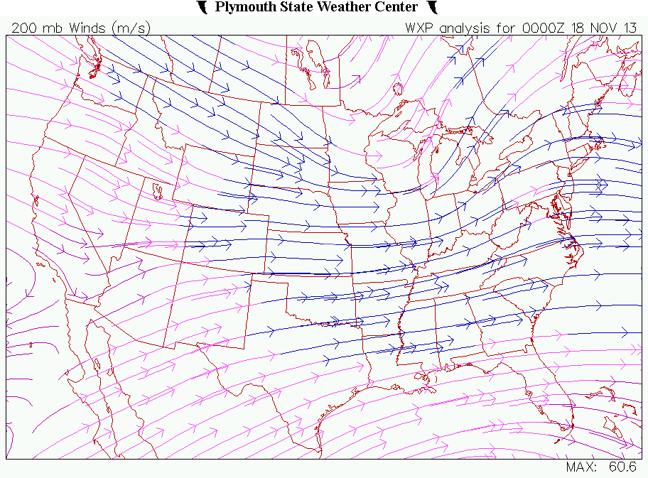
Figure 21b: This is a map showing streamlines, showing the direction from which the wind is coming and going to. The coloration shows where the wind is going the faster or slower. This map, 0z on the 18th, shows that there is an area of divergence occurring over Michigan, just out in front of the low pressure. (Plymouth state)
Figure 22a: This is the 500 hPa vorticity at 12Z on the 17th. The contour interval is every 20. There is a significant area of negative vorticity advection out in front of the vorticity. This would soon impact the low pressure by adding rotation to the atmosphere. (Gempak)
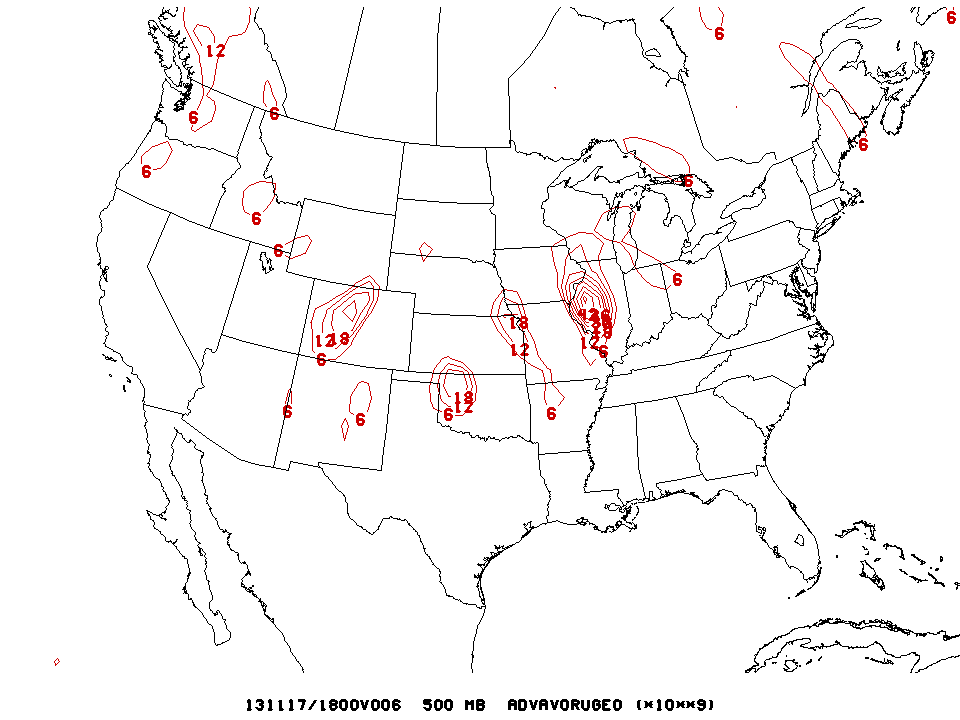
Figure 22b: This is 500 hPa vorticity at 18Z on the 17th, with contour interval of 6. The area that is seeing the vorticity advection is right behind the area that was seeing the convection. Downwind of the vorticity is an area of upward motion, adding to the potency of the storms (Gempak)
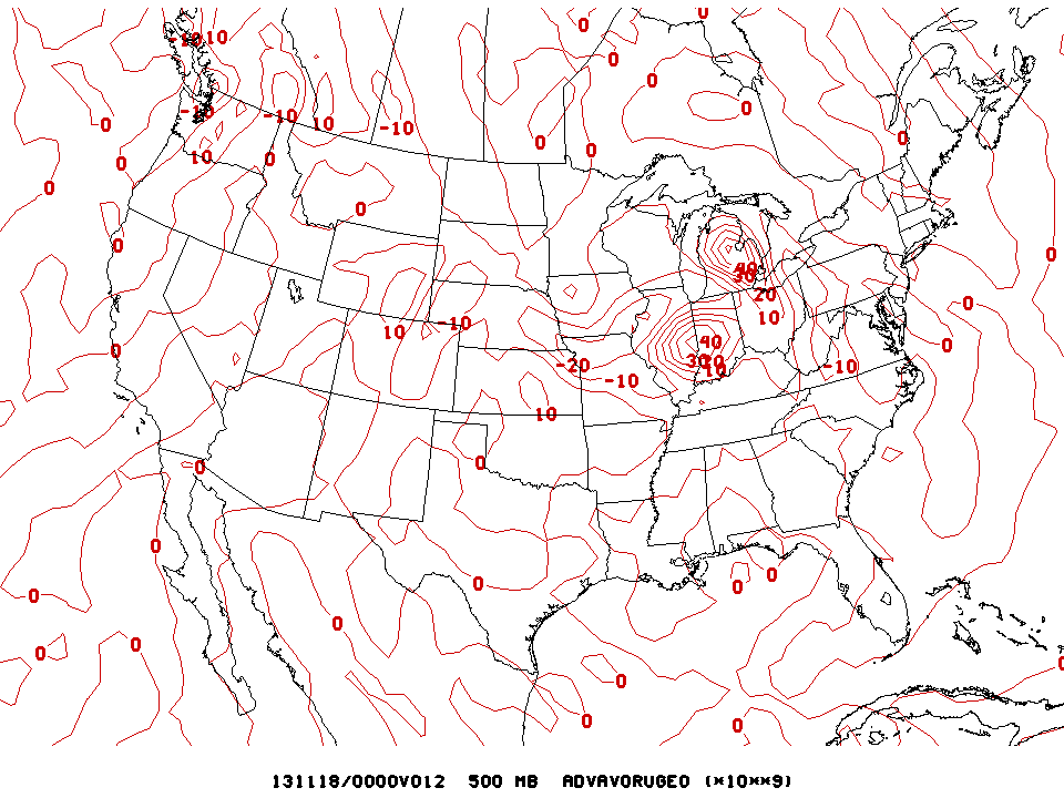
Figure 22c: This is 500 hPa vorticity at 0z on the 18th. The contour interval is at 10. An area of vorticity is seen over the state of Michigan, associated with the surface low pressure in the state. Further south, a second area of vorticity is seen over Indiana and eastern Illinois, strengthening the cold front as it moves eastward. (Gempak)
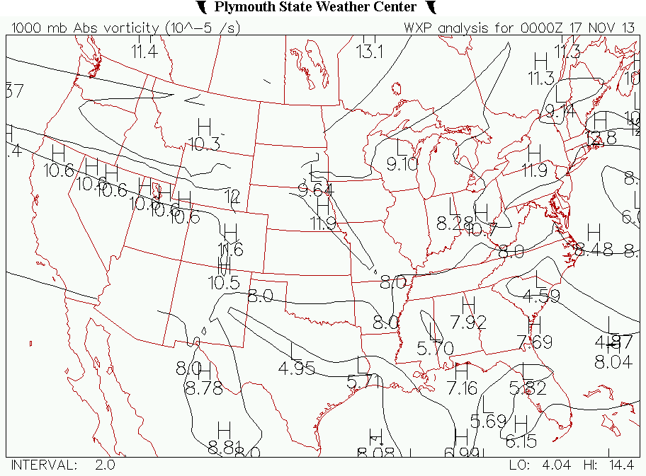
Figure 22d: This is the 1000 hPa absolute vorticity at 0Z on the 17th, with a contour value of 2. There is a maximum of vorticity over the eastern part of Nebraska. Downwind of a vorticity maximum there is upward motion. The low pressure at the surface was experiencing the upward motion from the vorticity at the surface. (Plymouth State)
Figure 22e: This is a map showing the absolute vorticity at 0Z on the 18th, with a contour interval of 2. The strongest lobe of vorticity is sitting over the northeastern corner of Illinois. This helped with the upward motion to strengthen the surface low pressure. (Plymouth state)
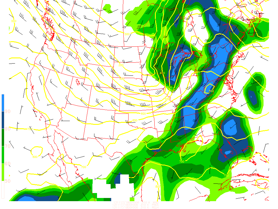 Figure 23a: This is a map depicting the isentropic surface of 310 kelvin at 18Z. On the map, we have wind barbs (the black pointers), pressure (the yellow contours, with a contour interval of every 50 hPa), and the relative humidity, with the areas that have the blue colors having the highest value of relative humidity at the 310K isosurface. The highest moisture advection at 310K was out in front of the frontal system with winds coming out of the southwest as well. This drew moisture from the Gulf of Mexico that the storm could use later on in its duration, along with the area of isentropic lifting north of the surface warm front, with moisture from the south gliding up and over the warm front. (Gempak)
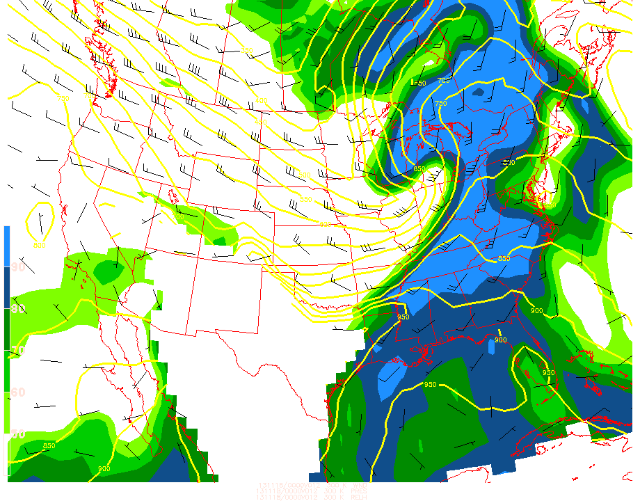
Figure 23b: This is a map depicting the isentropic surface at 300K at 0Z on the 18th. Much like the above isentropic surface, we have the wind barbs, pressure and relative humidity of the isentropic surface at that time. The area of deepest moisture at the 300K isosurface has moved eastward along the departing cold front. Winds out in front of the system were coming out of the southwest, with a switch on the backside of the low pressure to the northwest, which is what we expect to happen on the back side of a surface low. Of note is the large area of moisture in southern Canada, to the north of the positon of the warm front. This is where the isentropic lifting is occurring with this storm. (Gempak)
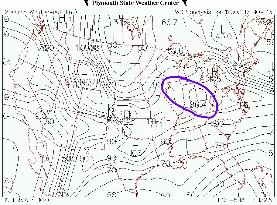
Figure 24: This the 250 hPa wind speed in knots, with a contour interval of 10 knots. The strongest a-geostrophic motion is out front of the jet streak where I added the blue circle. This area of a-geostrophic motion added upward motion to the atmosphere in the left exit region of the jet streak. (Plymouth State)
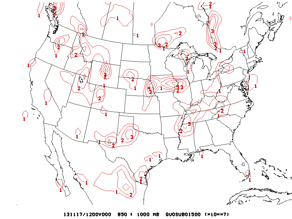
Figure 25a: This is omega at the 850-1000 hPa level, with a contour interval of 1. The strongest area of omega was associated with the area was just north of the warm front and the surface low. There was lifting occurring in this area, causing early morning convection along the warm front, and would also later help to enhance the upward motion needed for the convection. (Gempak)
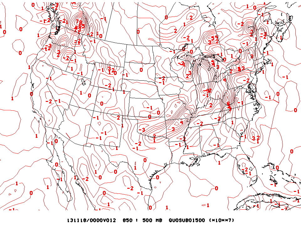
Figure 25b: This is omega at the 850-500 hPa levels, with a contour interval of 1. There is significant motion from omega over the Ark-La-Tex region, with another area further to the northeast. This helped with the upward motion needed for the convection to continue. (Gempak)
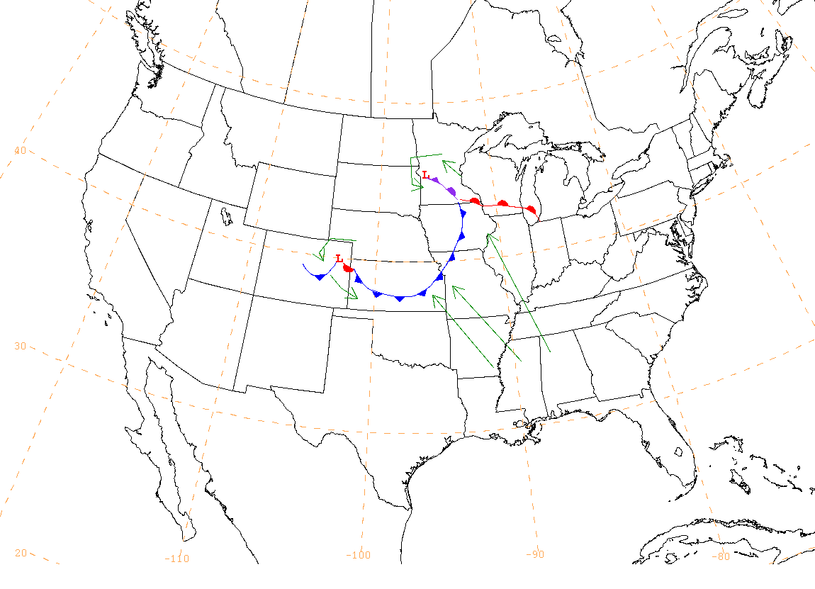
Figure 26: This is a conceptual model depicting the advection of moisture out ahead of the low pressure. As you can see, the storm system out ahead of the main low pressure was advecting moisture into itself, with the flow of moisture to the surface low over colorado really at a minimum due to the leading system doing a large majority of the moisture advection. (NMAP2)
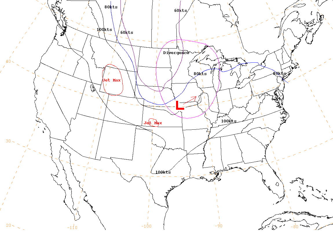
Figure 27: This is a conceptual model depicting the low pressure as it moved into the Northwestern portion of Missouri. It was under the influence of divergence at the 250 hPa level. This helped to deepen the low as it moved to the northeast. (NMAP2)
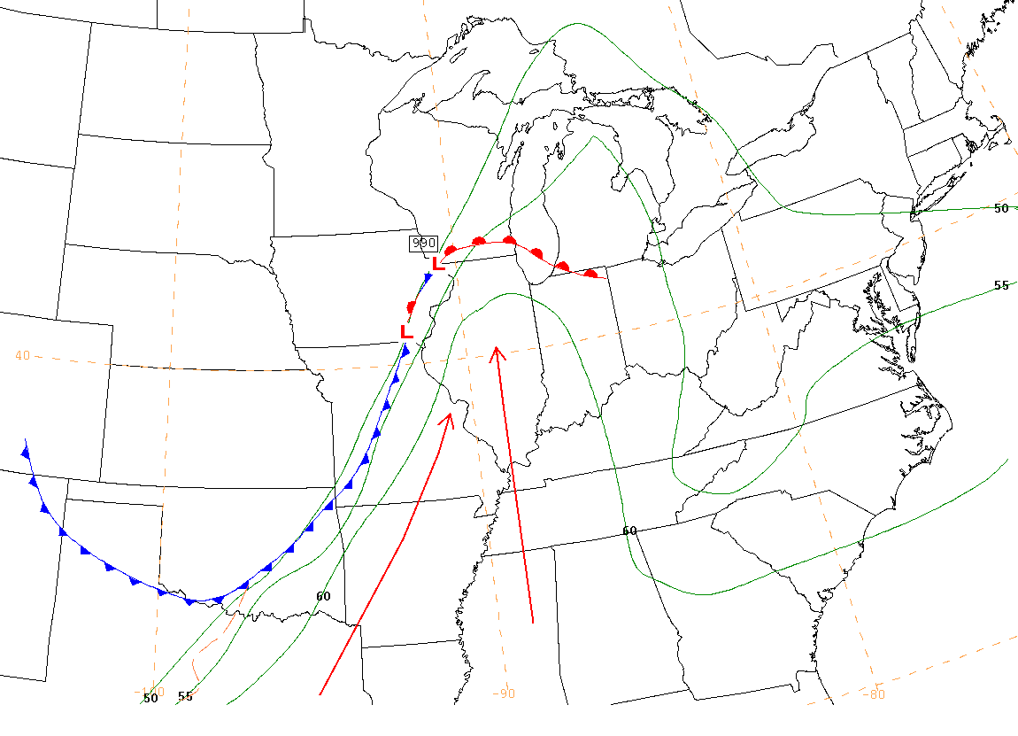
Figure 28: A conceptual model of the two low pressures now in Iowa. The southerly winds at the surface are pushing a surface warm front to the north. The green lines are isodrosotherms, lines of equal dew point temperature. This shows how far north the limited moisture that was in place went. (NMAP2)
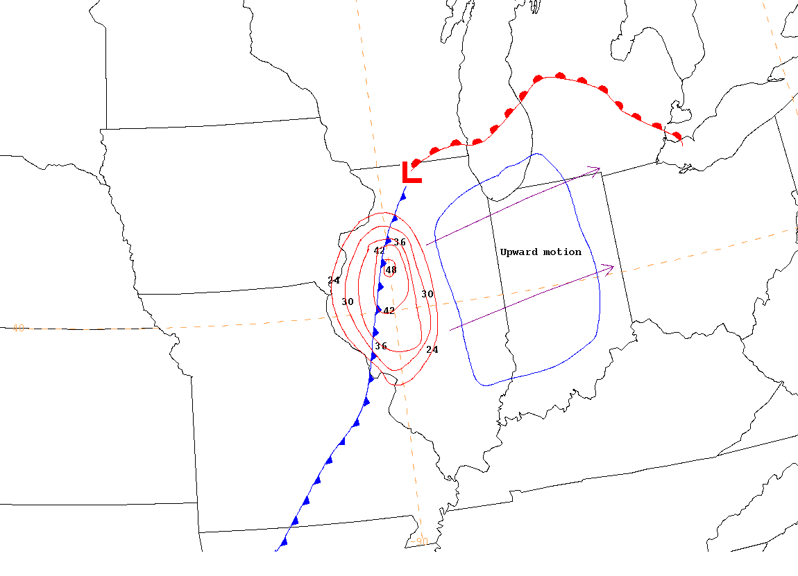
Figure 29: A conceptual model of the low pressure with the associated vorticity maximum. The vorticity max would move to the northeast, with upward motion to the east of the vort max. (NMAP2)